How to Get On Netflix

Are you an aspiring filmmaker? Are you intrigued by algorithms? Are you curious what aspects that companies and consumers look for in a successful movie? Then you’re in the right place. Today, I’m going to dive into what features of a movie make it most likely to be featured on Netflix. To figure this out, I conducted a binary classification model using data found on Kaggle (data updated as of May 2020). And the features of the data can be found below:

• Netflix: Whether the movie is found on Netflix
• ID: Arbitrary ID number for each movie
• Title: Title of the movie
• Year: The year in which the movie was produced
• IMDb: IMDb rating of the movie
• Rotten Tomatoes: Rotten Tomatoes % rating of the movie
• Hulu: Whether the movie is found on Hulu
• Prime Video Whether the movie is found on Amazon Prime Video
• Disney+ Whether the movie is found on Disney+
• Type: Is it a movie or a TV series
• Directors: Director of the movie
• Genres: Genre of the movie
• Country: Country origin of the movie
• Language: Primary language spoken in the movie
• Runtime: The runtime of the movie

Proofreading the Script

If we were to compare, creating a model, with producing a movie, one of the first steps would be to evaluate various scripts that writers send us. And if we found an appealing script, we would likely want to make edits to strike out the unnecessary plot holes, and expand upon the interesting plot points. Similarly, for creating a good classification model, using the data we received from Kaggle, we would need to trim the fat and delve deeper into the interesting points. And with a data set of 17,000 observations, one could imagine the amount of cleaning I had to do just to prepare the data for my model. So I took a nice and easy systematic approach to skimming some of the fat off my data.

Dropping High Null Count Features

My first step was to look at the null counts for all the features. To my dismay, I found that some of the more interesting features had high null counts. Both the Rotten Tomatoes (~11,500 null values) and Age (~9390 null values) had over half of their observations as null and had to be removed.

Dropping High-Cardinality and Low-Cardinality Features

Next I looked into which features had high-cardinality (had many unique values) and found three features that made the cut (Title, Directors, and ID). I wasn’t too sad about dropping these features because in terms of the greater picture of finding what movies/shows get on Netflix, these features would have little importance for prediction in our model. However, unfortunately, I found that Type seemed to be a broken feature in that it only had one value throughout (value = 0) and therefore had to be dropped since it would give no value to our model.

Dropping Irrelevant Features to Prevent Data Leakage

When I first created my model, I found that it was performing at absurd levels (>94% accuracy) and I had wondered why my model was overfitting. After taking a closer look at the features, I realized that some of my features were most likely causing data leakage and would need to be removed. I decided to remove Hulu, Prime Video, and Disney+ as it occurred to me that whether a movie/show was on Hulu, Amazon Prime, or Disney+ logically should have no bearing on whether a movie/show goes onto Netflix. It was also likely that a lot of movies/shows overlapped with Netflix, so there was data leakage that made my model overfit. However, I think it would be interesting to see what features matter most for the other streaming platforms and compare and contrast them in a future project.

Now that I dropped a lot of the fat, the features that would be incorporated in my model are the following:

• Netflix: Whether the movie is found on Netflix
• Year: The year in which the movie was produced
• IMDb: IMDb rating of the movie
• Genres: Genre of the movie
• Country: Country origin of the movie
• Language: Languages spoken in the movie
• Runtime: The runtime of the movie

Expanding the Interesting Scenarios

While exploring the data, I found that for three of my features, that some of their observations had multiple values that could be separated into new variables. For example, in the Language column, one observation could be ‘English, Japanese, Spanish’, which shows what languages were spoken in the film.

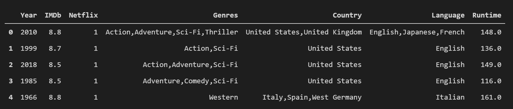
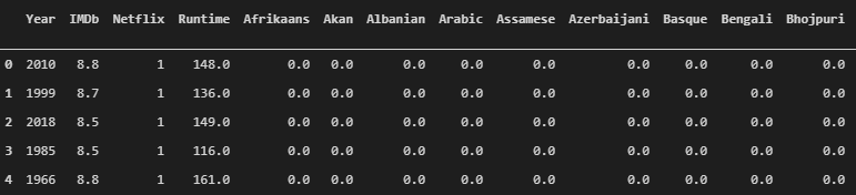
However, in order to tune our data so that our binary classification model performs better, it is better to convert these observations with multiple languages so that each language receives its own value. If you compare the image above to the image below, you can see now that the original Language column has been deleted, and replaced by each of the language values that it previously contained. So now, for the previous observation of ‘English, Japanese, Spanish’, there would be an int value of ‘1’ for the English, Japanese, and Spanish columns. I applied the same process for the Genres and Country columns as well, which expanded our dataframe to 201 columns(which still works since we still had 16,744 observations)

Hire the Crew to Get the Job Done

Now that we have our script written, it’s time to hire the producers, actors, and crew to create the movie. In our case, it’s finally time to build our model. Since our goal is to see what features help a movie get on Netflix, our target feature is Netflix. After using our target feature to create our training, validation, and test sets using a train_test_split, I wanted to use a random forest classification model and XGBoost model and see which model would create the best predictions and interesting feature importances. In order to check to see which model would be viable, I created a baseline accuracy, using the normalized max value of our y_train set that showed that the models had to beat a baseline accuracy of 78.9%. I would also look at other metrics of the models such as ROC AUC, precision, and recall scores to compare the efficacies of the models.

Random Forest Model

I first created a Random Forest model using randomized search and grid search methods to tune my hyper-parameters.

#Random Forest Model
model = make_pipeline(OrdinalEncoder(),
                      SimpleImputer(strategy = 'median'),
                      StandardScaler(),
                      RandomForestClassifier(random_state=42,
                                             max_depth = 60,
                                             n_estimators = 90,
                                             class_weight = 'balanced_subsample')
                      )
                                       
model.fit(X_train, y_train)

One hyper-parameter that I want to highlight is class_weight, which helps balance our unbalanced target Netflix. We previously saw in our baseline that the “0” value was far more heavily weighted (~78.9% of our data showed movies that weren’t on Netflix). Using the class_weight hyperparameter helps balance those weights so that we could increase our recall and precision values for our models down the line.

XGBoost Model

I also created an XGBoost Model and tuned the hyperparameters with randomized search methods. One different hyper-parameter is learning_rate, where a higher value helps increase the model fit (range is from 0 to 1)

#XGBoost Model
model_xgb = make_pipeline(OrdinalEncoder(),
                          SimpleImputer(strategy = 'median'),
                          XGBClassifier(random_state = 42,
                                        n_estimators=20,
                                        max_depth = 70,
                                        learning_rate= 0.00010526315789473685,
                                        n_jobs=-1))

model_xgb.fit(X_train, y_train)

Hosting a Screening of the Movie and Receiving Feedback

Now that we directed and produced the movie, it’s now time to hold a pre-release screening and see the initial reaction to our movie. Or in more technical terms, we fit our models and see what metrics we get from each model.

Accuracy of the Models

The first metric that we checked for both models is accuracy. We checked the accuracy of the Random Forest and XGBoost models for our training, validation, and test sets.

• Baseline Accuarcy : 0.789

• Random Forest Training Accuracy: 0.997
• Random Forest Validation Accuracy: 0.825

• Random Forest Testing Accuracy: 0.824

• XGBoost Accuracy Train: 0.894
• XGBoost Accuracy Val: 0.793
• XGBoost Accuracy Test: 0.807

We can see that both our models outperform our baseline which is a good sign. The main categories that concern ourselves with are how the models perform within the validation and testing sets, so I’m not too concerned with the high training accuracy for the Random Forest model. We also see that the Random Forest model performs better, and this is likely due to how we balanced the weights for the random forest model and not for the XGBoost model. Also to note, I previously had higher accuracy scores for my XGBoost model with other hyperparameters, however kept this version of the model as it had a more balanced recall and precision score.

Precision and Recall Values

Next, using the classification_report function from sklearn, I found the precision and recall values of the two models.

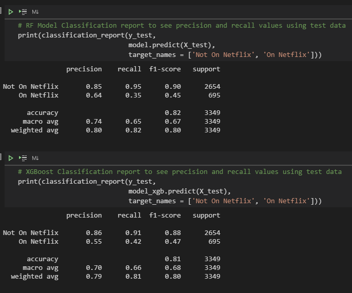
At first glance, we can see that the “Not On Netflix” precision and recall values are pretty high (>84%). This shows that our model was generally good at predicting movies that weren’t featured on Netflix. But however, more importantly, it seems that our “On Netflix” precision and recall values were much lower (35% - 64%). The precision values shows that of all the movies our model predicted to be on Netflix, what percentage of those predictions were correct (i.e., out of all the predictions our random forest model predicted to be on Netflix, it was correct for 64% of its guesses). The recall values shows that out of the total movies that were on Netflix, what percentage of those movies did our model correctly predict to be on Netflix (i.e., our random forest model predicted 35% of the total Netflix movies to be on Netflix). We can see that our XGBoost model slightly outperformed our random forest model, however, there is still a method to help increase our values.

Back to the Editing Room

Now that we got the initial response to our pre-release screening, it’s time to go back to the editing room and improve our film. In this case, we’re looking for a way to increase our relatively low precision and recall values for our random forest model. One way is to adjust our threshold values that our model uses to make predictions. Currently the default threshold value is at 50%, meaning if the model predicts the normalized value of “On Netflix’’ to be above 50%, it will predict that observation to be on Netflix. One way to see which threshold to choose, we can look at the ROC curve.

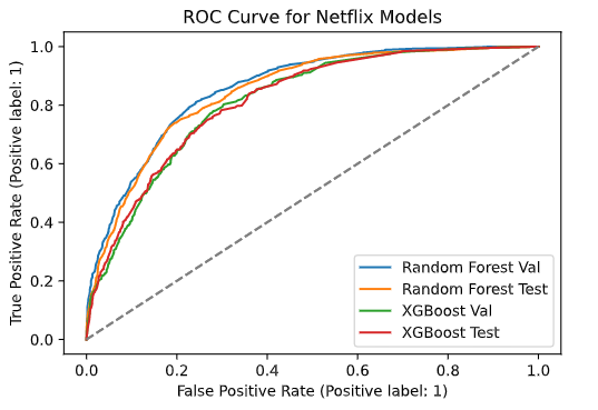
The ROC Curve compares the false positive rates (FPR) with the true positive rates (TPR) of our models. The ideal point on this model would be where there is a high true positive rate and a low false positive rate. Looking at the curve, we see the curve increase sharply at a high TPR at the FPR range of 0.1 - 0.3 before it starts to slowly taper off. This is the area where we want to see the corresponding threshold values. And by creating a mask, we are able to find the corresponding threshold to use to be 0.289. This threshold means that now instead of 50%, the model will predict the value of “On Netflix” to be equal to “1” if the normalized predicted y value is above 28.9%.

Release the Movie

Now that we re-edited the movie, it’s time to finally release it to theaters and hope for the best. So in data science terms, we use the new predicted values at the threshold of 0.289 and are able to create a new classification report to find new precision and recall values.

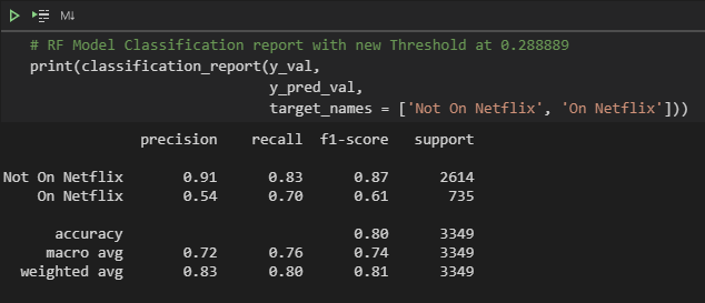
We can see in the above report that the precision and recall values increased significantly while the accuracy average is still above our baseline. Although, in a perfect world, I would ideally want a higher precision score as it’s still relatively low at 0.54, with my current knowledge of models, I’m happy with my results.

Most Important Features

Now that the movie is released, we can finally dive into answering our original question. What features are most important in a movie/show for Netflix to feature? Using python to extract the feature importances from my random forest model, I found the top 10 features below.

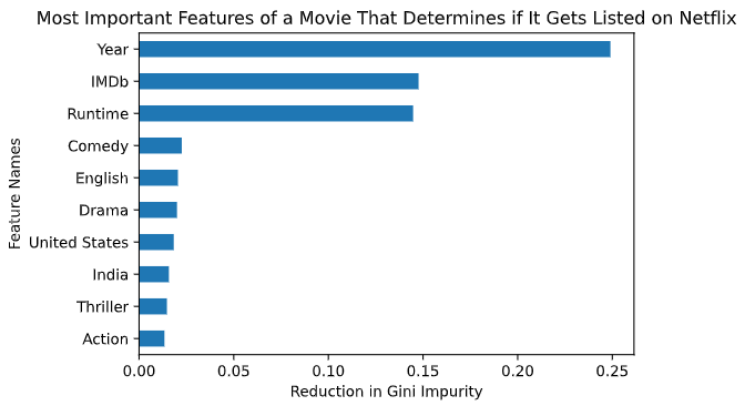
Looking at this graph, we can see by far the most important feature is the year the movie was produced. This shows that the newer the movie is, the more likely it would be featured on Netflix. Having a high IMDb rating is the second most important feature which logically makes sense. It also shows that a movie being produced in India has made it into our top 10 feature importances. It might be worth doing a deeper dive in the future to see Bollywood’s impact on Netflix.

Eh, What if I Don’t Care About Netflix?

Some of you might be reading this and wondering, so what? What if I don’t care about having my movie on Netflix, or on any other streaming platform for that matter. Then first, color me impressed that you even read this far. But second, I can also show you what features of a movie helps get a higher IMDb rating. In contrast to before, since an IMDb rating is a continuous numerical variable, I will be creating a Ridge Regression model to find the most important features for a high IMDb rating.

In terms of cleaning the data, it was very similar to what we did in the classification models. One change though is that we didn’t remove Hulu, Prime Video, and Disney+ features as I feel that they would be relevant for our ridge regression model.

The features that would be incorporated in my model are the following:

• Netflix: Whether the movie is found on Netflix
• Hulu: Whether the movie is found on Hulu
• Prime Video Whether the movie is found on Amazon Prime Video
• Disney+ Whether the movie is found on Disney+
• Year: The year in which the movie was produced
• IMDb: IMDb rating of the movie
• Genres: Genre of the movie
• Country: Country origin of the movie
• Language: Languages spoken in the movie
• Runtime: The runtime of the movie

After splitting the data, in order to get the baseline, I calculated the mean absolute error by using the mean of y_train and the predicted y values based on y. I found the baseline MAE to be 1.07. I then created a ridge regression model with the following hyperparameters.

# Ridge Regression Model
model = make_pipeline(OneHotEncoder(use_cat_names=True),
                      SimpleImputer(strategy = 'mean'),
                      StandardScaler(),
                      Ridge(alpha = 600),
                      )
                                             
model.fit(X_train, y_train)

Using the model, we found the MAE’s to be:

• Training MAE: 0.839
• Validation MAE: 0.856
• Test MAE: 0.874

Since these MAE’s are lower than our baseline, we can see that our ridge model is working well.

We also found the R-squared of the ridge regression model to be:

• Training R-squared: 0.351
• Validation R-squared: 0.331
• Test R-squared: 0.320

The R-squared values are pretty low overall, which most likely means that there are other features that we are unaware of that have an impact on IMDb rating. If we had a more expansive data set, we could perhaps improve the score with new features.

Even so, I was overall happy with the model, and therefore I pulled the coefficients from the features of the model to find most impactful features from this model.

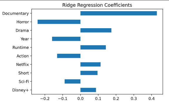
The main takeaways from these coefficients are that documentaries on average tend to have the highest IMDb scores while horror movies/shows tend to have the lowest IMDb scores. We can also see that movies being on Netflix have a positive impact on IMDb score. So maybe in the end, using a substantial leap in logic, aspiring filmmakers might want to make movies with a goal of being featured on Netflix to mind, in order to achieve a higher IMDb rating. On a more serious note, I hope you enjoyed seeing what features of a movie are impactful when trying to create a movie that’s featured on Netflix or achieve a higher IMDb rating.

Link to GitHub repo can be found here